Creating pivot table using Excel sheet

 Step By Step Procedure to create Pivot Tables:


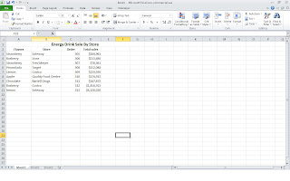
1. Open the Excel worksheet that contains the table you want summarized by pivot table and select any cell in the table.(Ensure that the table has no blank rows or columns and that each column has a header.)

Image 1

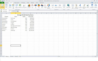
 2.Select the Insert tab. Click the top portion of the button for creating Pivot Tables OR  if you click the arrow, click PivotTable in the drop-down menu.(First from left side of the worksheet)

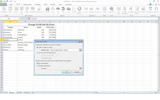
Excel opens the Create PivotTable dialog box and selects all the table data, as indicated by a marquee around the cell range.If necessary, adjust the range in the Table/Range text box under the Select a Table or Range option button. ( Make sure that you do not select the Heading. In the example below it is  "Energy Drink Sale By Store)

Image 2 

Image 3

 3. Select the location for the pivot table. By default, Excel builds the pivot table on a new worksheet it adds to the workbook. If you want the pivot table to appear on the same worksheet, click the Existing Worksheet option button and then indicate the location of the first cell of the new table in the Location text box. Enter the address of a cell that is a few rows below the data. ( For ex: A20 in the worksheet shown above)

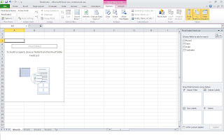
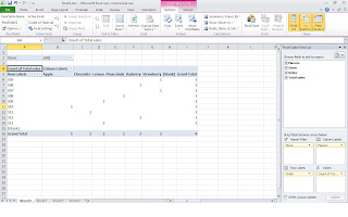
4. Excel  displays a "PivotTable Field List" task pane on the right side of the new worksheet . The PivotTable Field List task pane is divided into two areas.
    a)   The "Choose Fields to Add to Report"  list box with the names of all the fields in the source data for the pivot table.
    b)  An area divided into four drop zones (Report Filter, Column Labels, Row Labels, and Values) at the bottom.

Image 4

 5. To complete the pivot table, assign the fields in the PivotTable Field List task pane to the various parts of the table. You do this by dragging a field name from the Choose Fields to Add to Report list box and dropping it in one of the four areas below, called drop zones:

          a) Report Filter: This area contains the fields that enable you to page through the data summaries shown in the actual pivot table by filtering out sets of data — they act as the filters for the report. 

         b) Column Labels: This area contains the fields that determine the arrangement of data shown in the columns of the pivot table.

        c) Row Labels: This area contains the fields that determine the arrangement of data shown in the rows of the pivot table.

      d) Values: This area contains the fields that determine which data are presented in the cells of the pivot table — they are the values that are summarized in its last column (totaled by default).

Continue to manipulate the pivot table as needed until the desired results appear.

Image 5

Image 6

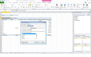
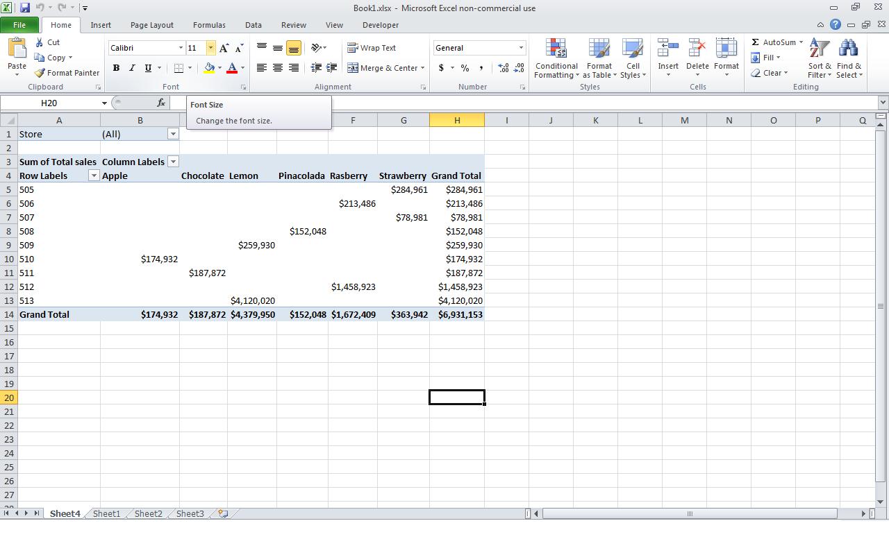
For the example  in Image 5 i had added  " Total sales" in " Values" area . Here you can see that it is taking it as count of numbers.To change it to currency, click on the Drop Down arrow of the " Sum of Totals" in the "Values" area. Then Select "Value field Setting". Under  " Summarize Value field by " select the option "Sum". Then to change it into Dollars or any Currency, select " Number Format" in the extreme left of the window. Here you can change it into currency as shown in Image 7.

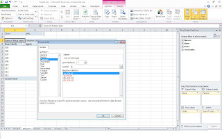Image 7

Your Simple Pivot Table is ready as shown in Image 8 below. To Edit the drop down Zone , just click on any cell in the tables and it will appear again.

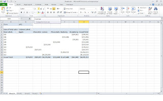Image 8

( Click on the Images to Enlarge it )